 Products Home
Polarization Camera with 5.0 MP Monochrome CMOS Sensor
- Polarization-Sensitive Monochrome CMOS Camera
- On-Chip Wire Grid Polarizer Array
- High Quantum Efficiency & Low <2.5 e- Read Noise
- C-Mount Compatible with 2/3" Optical Format
CS505MUP
Monochrome
Polarization Camera
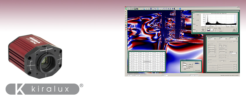
ThorCam software showing the calculated azimuth / angle of linear polarization (AoLP) of plastic safety goggles using the CS505MUP camera and polarized light. The captured image has a pseudocolor effect applied as a visualization aid. Click here to download the full-resolution image and see the Polarization tab below for more information.


Please Wait
| Scientific Camera Selection Guide | |
|---|---|
| Compact Scientific |
Zelux™ (Smallest Profile) |
| Kiralux® CMOS | |
| Kiralux® CMOS Polarization Sensitive | |
| Quantalux® (<1 e- Read Noise) |
|
| Scientific CCD | 1.4 MP CCD |
| 4 MP CCD | |
| 8 MP CCD | |
| VGA Resolution CCD (200 Frames Per Second) |
|
Applications
- Materials Inspection
- Stress Inspection
- Flaw Detection
- Contrast Improvement
- Transparent Material Detection
- Surface Reflection Reduction
- Depth Mapping

Jason Mills
General Manager,
Thorlabs Scientific Imaging
Feedback?
Questions?
Need a Quote?
Features
- Monochrome 5.0 MP CMOS Sensor with Integrated 4-Directional Wire Grid Polarizer Array
- High Quantum Efficiency: 72% from 525 to 580 nm (Typical)
- 3.45 µm x 3.45 µm Pixel Size
- Fan-Free, Passive Thermal Management Reduces Dark Current
Without Vibration and Image Blur - <2.5 e- RMS Read Noise (Unprocessed Images)
- Triggered and Bulb Exposure Modes
- Global Shutter
- USB 3.0 Interface
- ThorCam™ Software for Windows® 7 and 10 Operating Systems
- Available Polarization Imaging Modes:
- Intensity (Optical Power) / Stokes Vector S0
- Degree of Linear Polarization (DoLP; Shown in the Video Below)
- Azimuth / Angle of Linear Polarization (AoLP; Shown in the Screenshot Above)
- Unprocessed (Raw)
- QuadView (Unprocessed, Separated by Polarization)
- SDK and Programming Interface Support:
- C, C++, C#, Python, and Visual Basic .NET APIs
- LabVIEW, MATLAB, and µManager Third-Party Software
- Azimuth Orientation Engraved on Housing
- SM1-Threaded (1.035"-40) Aperture with Adapter for Standard C-Mount (1.000"-32)
- Compatible with 30 mm Cage System
- 1/4"-20 Tapped Holes for Post Mounting
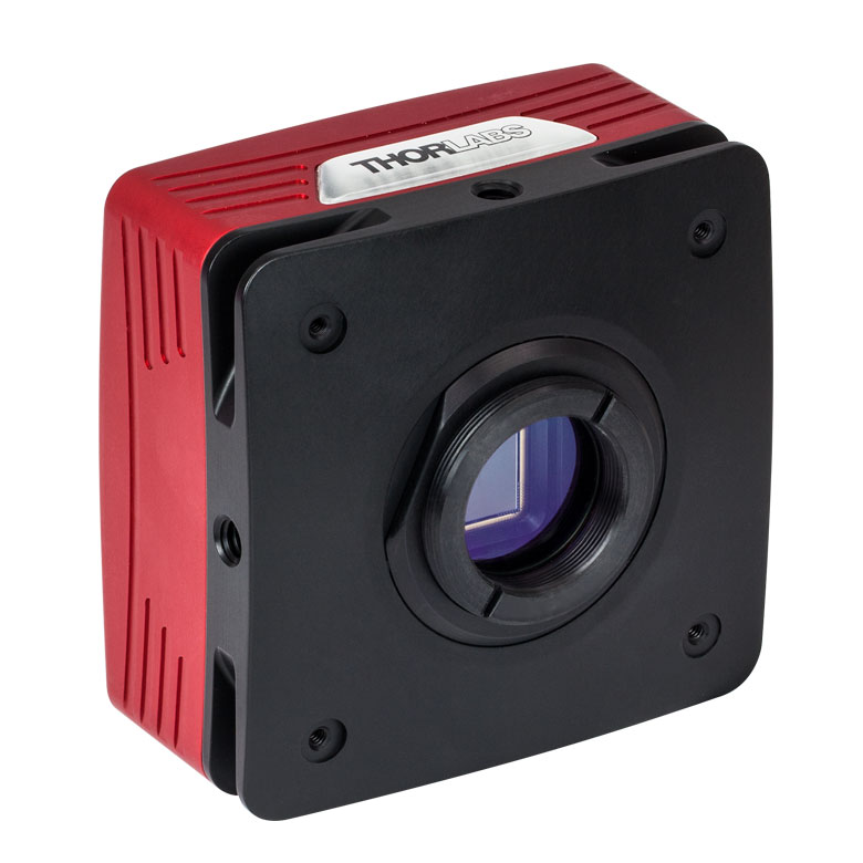
Thorlabs' Polarization-Sensitive Kiralux® Camera features a 5.0 MP monochrome CMOS sensor with a polarizer array. The wire grid polarizer array is comprised of a repeating pattern of polarizers (0°, 45°, -45°, and 90° transmission axes) and is present on the sensor chip between the microlens array and the photodiodes. The integrated polarizer array and software image processing enable the creation of images that illustrate degree of linear polarization (DoLP), azimuth, and intensity at the pixel level. These features enable many advanced techniques using polarization, for example: stress-induced birefringence detection, surface reflection reduction, materials inspection. The housing features engraved references for the polarization azimuth for ease of alignment.
This video of degree of linear polarization (DoLP, shown with false color) depicts the bending of a plastic handle imaged by our CS505MUP polarization camera and illuminated by polarized light. 16-bit images like the full-resolution image above may be viewed using ThorCam, ImageJ, or other scientific imaging software. They may not be displayed correctly in general-purpose image viewers.
The camera also offers extremely low read noise and high sensitivity for demanding imaging applications. The global shutter captures the entire field of view simultaneously, allowing for imaging of fast moving objects. The compact housing has been engineered to provide passive thermal management for the sensor, reducing dark current without the need for a cooling fan or thermoelectric cooler.
The approximate axial position of the sensor is indicated by the engraved line on top of the camera body. Each CMOS camera includes a USB 3.0 interface for compatibility with most computers. Included with each camera is our ThorCam software for use with Windows 7 and 10 operating systems. Developers can leverage our full-featured API and SDK. Visit the Thorcam Software page to download the latest software, firmware, and programing interfaces.
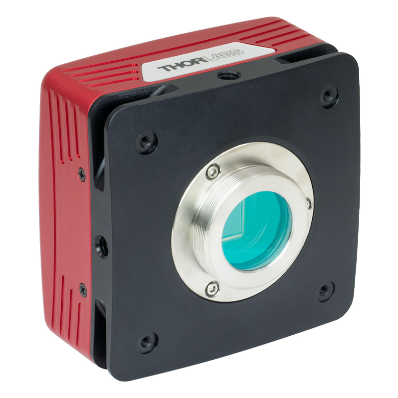
The camera aperture has SM1 (1.035"-40) threading for compatibility with Ø1" Lens Tubes; an adjustable C-Mount (1.000"-32) adapter is factory installed for out-of-the-box compatibility with many microscopes, machine vision camera lenses, and C-Mount extension tubes. A replacement C-Mount adapter, SM1A10A, is available separately below. Each monochrome camera features a protective window. This window can be removed and replaced with another Ø25 mm or Ø1" optic up to 1.27 mm thick when using the camera's C-mount adapter. Without this adapter, the maximum filter thickness is 4.4 mm.
Four 4-40 tapped holes provide compatibility with our 30 mm cage system. Two 1/4"-20 tapped holes on opposite sides of the housing are compatible with imperial Ø1" pedestal or pillar posts. The combination of flexible mounting options and compact size makes these CMOS cameras the ideal choice for integrating into custom-built imaging systems as well as those based on commercial microscopes.
Camera Mounting Features |
||||
 Click to Enlarge Removing the C-Mount adapter and locking ring exposes the SM1 (1.035"-40) threading that can be used for custom assemblies using standard Thorlabs components. |
 Click to Enlarge An SM1 Lens Tube installed using the SM1-threaded aperture. |
 Click to Enlarge Four 4-40 tapped holes allow 30 mm Cage System components to be attached to the camera. Pictured is our CP13 Cage Plate with C-Mount Threading. |
||

| Item #a | CS505MUP |
|---|---|
| Sensor Type | Monochrome CMOS with Wire Grid Polarizer Arrayb |
| Effective Number of Pixels (Horizontal x Vertical) |
2448 x 2048 |
| Imaging Area (Horizontal x Vertical) | 8.4456 mm x 7.0656 mm |
| Pixel Size | 3.45 µm x 3.45 µm |
| Optical Format | 2/3" (11 mm Diagonal) |
| Max Frame Rate | 35 fps (Full Sensor) |
| ADCc Resolution | 12 Bits |
| Sensor Shutter Type | Global |
| Peak Quantum Efficiency | 72% from 525 to 580 nm (Typical) |
| Read Noise | <2.5 e- RMSd |
| Full Well Capacity | ≥10 000 e- |
| Exposure Time | 0.027 ms to 14235 ms in ~0.013 ms Increments |
| Vertical and Horizontal Hardware Binning | 1 x 1 to 16 x 16 |
| Region of Interest (ROI) | 260 x 4 Pixelse to 2448 x 2048 Pixels, Rectangular |
| Dynamic Range | Up to 71 dB |
| Lens Mount | C-Mount (1.000"-32) |
| Mounting Features | Two 1/4"-20 Taps for Post Mounting 30 mm Cage Compatible |
| Removable Optic | Window, Ravg < 0.5% per Surface (400 - 700 nm) |
| USB Power Consumption | 3.6 W @ 35 fps (Full Sensor ROI) |
| Ambient Operating Temperature | 10 °C to 40 °C (Non-Condensing) |
| Storage Temperature | 0 °C to 55 °C |
| Example Frame Rates at 1 ms Exposure Timea,b | |
|---|---|
| Region of Interest | Frame Rate |
| Full Sensor (2448 x 2048) | 35 fps |
| Half Sensor (1224 x 1024) | 68 fps |
| ~1/10 Sensor (260 x 208) | 290 fps |
| Minimum ROI (260 x 4) | 887.6 fps |

Click to Enlarge
Mechanical Drawing of the Kiralux® Camera Housing


Click to Enlarge
Click for Raw Data
This curve shows the extinction ratio (ER) for the on-chip, four-directional wire grid polarizer array. The extinction ratio is the ratio of maximum to minimum transmission of a sufficiently linearly polarized input. When the transmission axis and input polarization are parallel, the transmission is at its maximum; rotate the polarizer by 90° for minimum transmission.

Click to Enlarge
The wire grid polarizer array is comprised of a repeating polarizer pattern (0°, 45°, -45°, and 90°) and is present on the sensor chip between the microlens array and the photodiodes. Integrating the polarizers between the microlenses and photodiodes minimizes the crosstalk between adjacent polarizers and increase alignment accuracy compared to a polarizer array placed in front of the microlens array.
Click to Enlarge
The four-directional wire grid polarizer array is present on the sensor chip between the microlens array and the photodiodes.

Click to Enlarge
Wire grid polarizers transmit radiation with an electric field vector perpendicular to the wire and reflect radiation with the electric field-vector parallel to the wire
Polarization Features
- CMOS Sensor with Integrated 4-Directional Wire Grid Polarizer Array
- ThorCam™ Software Polarization Imaging Modes:
- Intensity (Optical Power) / Stokes Vector S0
- Degree of Linear Polarization (DoLP)
- Azimuth / Angle of Linear Polarization (AoLP)
- Unprocessed (Raw)
- QuadView (Unprocessed, Separated by Polarization)
The CS505MUP polarization camera's image sensor incorporates an integrated, linear micropolarizer array to detect the linear polarization states within the image. Integrating the polarizers between the microlenses and photodiodes minimizes crosstalk and increases alignment accuracy between the polarizer orientations and their respective pixels compared to a polarizer array placed in front of the microlens array. The polarizer array is composed of wire grid polarizers fabricated directly on the sensor and arranged in a mosaic pattern, as shown in the drawing to the far right. These polarizers consist of an array of parallel metallic wires that transmit radiation with an electric field vector perpendicular to the wire and reflect radiation with the electric field-vector parallel to the wire, as illustrated in the drawing above. Each pixel is covered with one of four linear polarizers with orientations of -45°, 0°, 45°, or 90°. These pixel values are then used to compute the three polarization parameters for the light incident at every pixel: intensity, degree of linear polarization, and azimuth.
The images below depict the hinge on a pair of plastic safety glasses and reflection reduction on a vehicle windshield. The upper left image was acquired in intensity mode, while the upper right and lower left software screenshots were taken in DoLP and azimuth image modes. Refer to the ThorCam user guide (included with the software documentation or accessible through the Support Docs (![]() ) icon below) for more information on operating the polarization camera and interacting with polarization images. Note that images are saved in the image type selected and include any processing that the image type applies. Save images in Unprocessed or QuadView modes if separate processing is necessary.
) icon below) for more information on operating the polarization camera and interacting with polarization images. Note that images are saved in the image type selected and include any processing that the image type applies. Save images in Unprocessed or QuadView modes if separate processing is necessary.
Note that high-bit-depth images like the full-resolution images available for download below may be viewed using ThorCam, ImageJ, or other scientific imaging software. They may not be displayed correctly in general-purpose image viewers.

Click to Enlarge
Intensity Image of Hinge on a Pair of Plastic Glasses
Click Here to View the Full-Resolution Image

Click to Enlarge
ThorCam Screenshot of Degree of Linear Polarization View
Click Here to View the Full-Resolution Image


Click to Enlarge
ThorCam Screenshot of QuadView
Camera Back Panel Connector Locations

For the I/O connector pin assignments, please see the Auxiliary (I/O) Connector section below.
TSI-IOBOB and TSI-IOBOB2 Break-Out Board Connector Locations

Click to Enlarge
TSI-IOBOB

Click to Enlarge
TSI-IOBOB2
| TSI-IOBOB and TSI-IOBOB2 Connector | 8050-CAB1 Connectors | Camera Auxiliary (I/O) Port |
|---|---|---|
 Female 6-Pin Mini Din Female Connector |
 Male 6-Pin Mini Din Male Connector (TSI-IOBOB end of Cable)  Male 12-Pin Hirose Connector (Camera end of Cable) |
 Female 12-Pin Hirose Connector (Auxiliary Port on Camera) |
Auxiliary (I/O) Connector
The camera and the break-out boards feature female connectors; the camera has a 12 pin Hirose connector, while the break out boards have a 6-pin Mini-DIN connector. The 8050-CAB1 cable features male connectors on both ends: a 12-pin connector for connecting to the camera and a 6-pin Mini-DIN connector for the break-out boards. Pins 1, 2, 3, 5, and 6 are each connected to the center pin of an SMA connector on the break-out boards, while pin 4 (ground) is connected to each SMA connector housing. To access one of the I/O functions not available with the 8050-CAB1, the user must fabricate a cable using shielded cabling in order for the camera to adhere to CE and FCC compliance; additional details are provided in the camera manual.
| Camera I/O Pin # |
TSI-IOBOB and TSI-IOBOB2 Pin # |
Signal | Description |
|---|---|---|---|
| 1 | - | GND | The electrical ground for the camera signals. |
| 2 | - | GND | The electrical ground for the camera signals. |
| 3 | - | GND | The electrical ground for the camera signals. |
| 4 | 6 | STROBE_OUT (Output) |
An LVTTL output that is high during the actual sensor exposure time when in continuous, overlapped exposure mode. It is typically used to synchronize an external flash lamp or other device with the camera. |
| 5 | 3 | TRIGGER_IN (Input) |
An LVTTL input used to trigger exposures. Transitions can occur from the high to low state or from the low to high state as selected in ThorCam; the default is low to high. |
| 6 | 1 | LVAL_OUT (Output) |
Refers to "Line Valid." It is an active-high LVTTL signal and is asserted during the valid pixel period on each line. It returns low during the inter-line period between each line and during the inter-frame period between each frame. |
| 7 | - | OPTO I/O_OUT STROBE (Output) |
This is an optically isolated output signal. The user must provide a pull-up resistor to an external voltage source of 2.5 V to 20 V. The pull-up resistor must limit the current into this pin to <40 mA. The default signal present on pin 7 is the STROBE_OUT signal, which is effectively the Trigger Out signal as well. |
| 8 | - | OPTO I/O_RTN | This is the return connection for the OPTO I/O_OUT output and the OPTO I/O_IN input connections. This must be connected to the pull-up source for OPTO I/O_OUT or the driving source for the OPTO I/O_IN signals. |
| 9 | - | OPTO I/O_IN (Input) |
This is an optically isolated input signal used to trigger exposures. The user must provide a driving source from 3.3 V to 10 V. An internal series resistor limits the current to <50 mA at 10 V. |
| 10 | 4 | GND | The electrical ground for the camera signals. |
| 11 | - | GND | The electrical ground for the camera signals. |
| 12 | 5 | FVAL_OUT (Output) |
Refers to "Frame Valid." It is a LVTTL output that is high during active readout lines and returns low between frames. |

Click to Enlarge
Compact Scientific Camera with Included Accessories
The following accessories are included with each Compact Scientific Camera:
- USB 3.0 Cable (Micro B to A)
- Wrench to Loosen Optical Assembly (Item # SPW502)
- Lens Mount Dust Cap
- CD with ThorCam Software
- Quick-Start Guide and Manual Download Information Card
ThorCam™
ThorCam is a powerful image acquisition software package that is designed for use with our cameras on 32- and 64-bit Windows® 7 or 10 systems. This intuitive, easy-to-use graphical interface provides camera control as well as the ability to acquire and play back images. Single image capture and image sequences are supported. Please refer to the screenshots below for an overview of the software's basic functionality.
Application programming interfaces (APIs) and a software development kit (SDK) are included for the development of custom applications by OEMs and developers. The SDK provides easy integration with a wide variety of programming languages, such as C, C++, C#, Python, and Visual Basic .NET. Support for third-party software packages, such as LabVIEW, MATLAB, and µManager* is available. We also offer example Arduino code for integration with our TSI-IOBOB2 Interconnect Break-Out Board.
*µManager control of Zelux and 1.3 MP Kiralux cameras is not currently supported. When controlling the Kiralux Polarization-Sensitive Camera using µManager, only intensity images can be taken; the ThorCam software is required to produce images with polarization information.
| Recommended System Requirementsa | |
|---|---|
| Operating System | Windows® 7 or 10 (64 Bit) |
| Processor (CPU)b | ≥3.0 GHz Intel Core (i5 or Higher) |
| Memory (RAM) | ≥8 GB |
| Hard Drivec | ≥500 GB (SATA) Solid State Drive (SSD) |
| Graphics Cardd | Dedicated Adapter with ≥256 MB RAM |
| Motherboard | USB 3.0 (-USB) Cameras: Integrated Intel USB 3.0 Controller or One Unused PCIe x1 Slot (for Item # USB3-PCIE) GigE (-GE) Cameras: One Unused PCIe x1 Slot |
| Connectivity | USB or Internet Connectivity for Driver Installation |
Software
Version 3.5.1
Click the button below to visit the ThorCam software page.
Example Arduino Code for TSI-IOBOB2 Board
Click the button below to visit the download page for the sample Arduino programs for the TSI-IOBOB2 Shield for Arduino. Three sample programs are offered:
- Trigger the Camera at a Rate of 1 Hz
- Trigger the Camera at the Fastest Possible Rate
- Use the Direct AVR Port Mappings from the Arduino to Monitor Camera State and Trigger Acquisition
Click the Highlighted Regions to Explore ThorCam Features

Camera Control and Image Acquisition
Camera Control and Image Acquisition functions are carried out through the icons along the top of the window, highlighted in orange in the image above. Camera parameters may be set in the popup window that appears upon clicking on the Tools icon. The Snapshot button allows a single image to be acquired using the current camera settings.
The Start and Stop capture buttons begin image capture according to the camera settings, including triggered imaging.
Timed Series and Review of Image Series
The Timed Series control, shown in Figure 1, allows time-lapse images to be recorded. Simply set the total number of images and the time delay in between captures. The output will be saved in a multi-page TIFF file in order to preserve the high-precision, unaltered image data. Controls within ThorCam allow the user to play the sequence of images or step through them frame by frame.
Measurement and Annotation
As shown in the yellow highlighted regions in the image above, ThorCam has a number of built-in annotation and measurement functions to help analyze images after they have been acquired. Lines, rectangles, circles, and freehand shapes can be drawn on the image. Text can be entered to annotate marked locations. A measurement mode allows the user to determine the distance between points of interest.
The features in the red, green, and blue highlighted regions of the image above can be used to display information about both live and captured images.
ThorCam also features a tally counter that allows the user to mark points of interest in the image and tally the number of points marked (see Figure 2). A crosshair target that is locked to the center of the image can be enabled to provide a point of reference.
Third-Party Applications and Support
ThorCam is bundled with support for third-party software packages such as LabVIEW, MATLAB, and .NET. Both 32- and 64-bit versions of LabVIEW and MATLAB are supported. A full-featured and well-documented API, included with our cameras, makes it convenient to develop fully customized applications in an efficient manner, while also providing the ability to migrate through our product line without having to rewrite an application.

Click to Enlarge
Figure 1: A timed series of 10 images taken at 1 second intervals is saved as a multipage TIFF.

Click to Enlarge
Figure 2: A screenshot of the ThorCam software showing some of the analysis and annotation features. The Tally function was used to mark four locations in the image. A blue crosshair target is enabled and locked to the center of the image to provide a point of reference.
Performance Considerations
Please note that system performance limitations can lead to "dropped frames" when image sequences are saved to the disk. The ability of the host system to keep up with the camera's output data stream is dependent on multiple aspects of the host system. Note that the use of a USB hub may impact performance. A dedicated connection to the PC is preferred. USB 2.0 connections are not supported.
First, it is important to distinguish between the frame rate of the camera and the ability of the host computer to keep up with the task of displaying images or streaming to the disk without dropping frames. The frame rate of the camera is a function of exposure and readout (e.g. clock, ROI) parameters. Based on the acquisition parameters chosen by the user, the camera timing emulates a digital counter that will generate a certain number of frames per second. When displaying images, this data is handled by the graphics system of the computer; when saving images and movies, this data is streamed to disk. If the hard drive is not fast enough, this will result in dropped frames.
One solution to this problem is to ensure that a solid state drive (SSD) is used. This usually resolves the issue if the other specifications of the PC are sufficient. Note that the write speed of the SSD must be sufficient to handle the data throughput.
Larger format images at higher frame rates sometimes require additional speed. In these cases users can consider implementing a RAID0 configuration using multiple SSDs or setting up a RAM drive. While the latter option limits the storage space to the RAM on the PC, this is the fastest option available. ImDisk is one example of a free RAM disk software package. It is important to note that RAM drives use volatile memory. Hence it is critical to ensure that the data is moved from the RAM drive to a physical hard drive before restarting or shutting down the computer to avoid data loss.
Triggered Camera Operation
Our scientific cameras have three externally triggered operating modes: streaming overlapped exposure, asynchronous triggered acquisition, and bulb exposure driven by an externally generated trigger pulse. The trigger modes operate independently of the readout (e.g., binning) settings as well as gain and offset. Figures 1 through 3 show the timing diagrams for these trigger modes, assuming an active low external TTL trigger.

Click to Enlarge
Figure 1: Streaming overlapped exposure mode. When the external trigger goes low, the exposure begins, and continues for the software-selected exposure time, followed by the readout. This sequence then repeats at the set time interval. Subsequent external triggers are ignored until the camera operation is halted. For the definition of the TTL signals, please see the Pin Diagrams tab.

Click to Enlarge
Figure 2: Asynchronous triggered acquisition mode. When the external trigger signal goes low, an exposure begins for the preset time, and then the exposure is read out of the camera. During the readout time, the external trigger is ignored. Once a single readout is complete, the camera will begin the next exposure only when the external trigger signal goes low.

Click to Enlarge
Figure 3: Bulb exposure mode. The exposure begins when the external trigger signal goes low and ends when the external trigger signal goes high. Trigger signals during camera readout are ignored.
Camera Specific Timing Considerations
Due to the general operation of our CMOS sensor cameras, as well as typical system propagation delays, the timing relationships shown above are subject to the following considerations:
- The delay from the external trigger to the start of the exposure and strobe signals is typically 270 ns for all triggered modes (standard and PDX/Bulb).
- For PDX/Bulb mode triggered exposures, in addition to the 270 ns delay at the start of the exposure, there is also a 13.72 µs integration period AFTER the falling edge of the external trigger. This is inherent in the sensor operation. It is important to note that the Strobe_out signal includes the additional 13.72 µs integration time and therefore is a better representation of the actual exposure time. Our suggestion is to use the Strobe_out signal to measure your exposure time and adjust your PDX mode trigger pulse accordingly.
External Triggering

Click to Enlarge
Figure 4: The ThorCam Camera Settings window. The red and blue highlighted regions indicate the trigger settings as described in the text.
External triggering enables these cameras to be easily integrated into systems that require the camera to be synchronized to external events. The Strobe Output goes high to indicate exposure; the strobe signal may be used in designing a system to synchronize external devices to the camera exposure. External triggering requires a connection to the auxiliary port of the camera. We offer the 8050-CAB1 auxiliary cable as an optional accessory. Two options are provided to "break out" individual signals. The TSI-IOBOB provides SMA connectors for each individual signal. Alternately, the TSI-IOBOB2 also provides the SMA connectors with the added functionality of a shield for Arduino boards that allows control of other peripheral equipment. More details on these three optional accessories are provided below.
Trigger settings are adjusted using the ThorCam software. Figure 4 shows the Camera Settings window, with the trigger settings highlighted with red and blue squares. Settings can be adjusted as follows:
- "Hardware Trigger" (Red Highlight) Set to "None": The camera will simply acquire the number of frames in the "Frames per Trigger" box when the capture button is pressed in ThorCam.
- "Hardware Trigger" Set to "Standard": There are Two Possible Scenarios:
- "Frames per Trigger" (Blue Highlight) Set to Zero or >1: The camera will operate in streaming overlapped exposure mode (Figure 1).
- "Frames per Trigger" Set to 1: Then the camera will operate in asynchronous triggered acquisition mode (Figure 2).
- "Hardware Trigger" Set to "Bulb (PDX) Mode": The camera will operate in bulb exposure mode, also known as Pulse Driven Exposure (PDX) mode (Figure 3).
In addition, the polarity of the trigger can be set to "On High" (exposure begins on the rising edge) or "On Low" (exposure begins on the falling edge) in the "Hardware Trigger Polarity" box (highlighted in red in Figure 4).
Example Camera Triggering Configuration using Scientific Camera Accessories

Figure 5: A schematic showing a system using the TSI-IOBOB2 to facilitate system integration and control.
While the diagram shows the back panel of our Quantalux™ sCMOS Camera, our Scientific CCD cameras can be used as well.
As an example of how camera triggering can be integrated into system control is shown in Figure 5. In the schematic, the camera is connected to the TSI-IOBOB2 break-out board / shield for Arduino using a 8050-CAB1 cable. The pins on the shield can be used to deliver signals to simultaneously control other peripheral devices, such as light sources, shutters, or motion control devices. Once the control program is written to the Arduino board, the USB connection to the host PC can be removed, allowing for a stand-alone system control platform; alternately, the USB connection can be left in place to allow for two-way communication between the Arduino and the PC. Configuring the external trigger mode is done using ThorCam as described above.

Insights into Mounting Lenses to Thorlabs' Scientific Cameras
Scroll down to read about compatibility between lenses and cameras of different mount types, with a focus on Thorlabs' scientific cameras.
- Can C-mount and CS-mount cameras and lenses be used with each other?
- Do Thorlabs' scientific cameras need an adapter?
- Why can the FFD be smaller than the distance separating the camera's flange and sensor?
Click here for more insights into lab practices and equipment.
Can C-mount and CS-mount cameras and lenses be used with each other?

Click to Enlarge
Figure 1: C-mount lenses and cameras have the same flange focal distance (FFD), 17.526 mm. This ensures light through the lens focuses on the camera's sensor. Both components have 1.000"-32 threads, sometimes referred to as "C-mount threads".

Click to Enlarge
Figure 2: CS-mount lenses and cameras have the same flange focal distance (FFD), 12.526 mm. This ensures light through the lens focuses on the camera's sensor. Their 1.000"-32 threads are identical to threads on C-mount components, sometimes referred to as "C-mount threads."
The C-mount and CS-mount camera system standards both include 1.000"-32 threads, but the two mount types have different flange focal distances (FFD, also known as flange focal depth, flange focal length, register, flange back distance, and flange-to-film distance). The FFD is 17.526 mm for the C-mount and 12.526 mm for the CS-mount (Figures 1 and 2, respectively).
Since their flange focal distances are different, the C-mount and CS-mount components are not directly interchangeable. However, with an adapter, it is possible to use a C-mount lens with a CS-mount camera.
Mixing and Matching
C-mount and CS-mount components have identical threads, but lenses and cameras of different mount types should not be directly attached to one another. If this is done, the lens' focal plane will not coincide with the camera's sensor plane due to the difference in FFD, and the image will be blurry.
With an adapter, a C-mount lens can be used with a CS-mount camera (Figures 3 and 4). The adapter increases the separation between the lens and the camera's sensor by 5.0 mm, to ensure the lens' focal plane aligns with the camera's sensor plane.
In contrast, the shorter FFD of CS-mount lenses makes them incompatible for use with C-mount cameras (Figure 5). The lens and camera housings prevent the lens from mounting close enough to the camera sensor to provide an in-focus image, and no adapter can bring the lens closer.
It is critical to check the lens and camera parameters to determine whether the components are compatible, an adapter is required, or the components cannot be made compatible.
1.000"-32 Threads
Imperial threads are properly described by their diameter and the number of threads per inch (TPI). In the case of both these mounts, the thread diameter is 1.000" and the TPI is 32. Due to the prevalence of C-mount devices, the 1.000"-32 thread is sometimes referred to as a "C-mount thread." Using this term can cause confusion, since CS-mount devices have the same threads.
Measuring Flange Focal Distance
Measurements of flange focal distance are given for both lenses and cameras. In the case of lenses, the FFD is measured from the lens' flange surface (Figures 1 and 2) to its focal plane. The flange surface follows the lens' planar back face and intersects the base of the external 1.000"-32 threads. In cameras, the FFD is measured from the camera's front face to the sensor plane. When the lens is mounted on the camera without an adapter, the flange surfaces on the camera front face and lens back face are brought into contact.

Click to Enlarge
Figure 5: A CS-mount lens is not directly compatible with a C-mount camera, since the light focuses before the camera's sensor. Adapters are not useful, since the solution would require shrinking the flange focal distance of the camera (blue arrow).

Click to Enlarge
Figure 4: An adapter with the proper thickness moves the C-mount lens away from the CS-mount camera's sensor by an optimal amount, which is indicated by the length of the purple arrow. This allows the lens to focus light on the camera's sensor, despite the difference in FFD.

Click to Enlarge
Figure 3: A C-mount lens and a CS-mount camera are not directly compatible, since their flange focal distances, indicated by the blue and yellow arrows, respectively, are different. This arrangement will result in blurry images, since the light will not focus on the camera's sensor.
Date of Last Edit: July 21, 2020
Do Thorlabs' scientific cameras need an adapter?

Click to Enlarge
Figure 6: An adapter can be used to optimally position a C-mount lens on a camera whose flange focal distance is less than 17.526 mm. This sketch is based on a Zelux camera and its SM1A10Z adapter.

Click to Enlarge
Figure 7: An adapter can be used to optimally position a CS-mount lens on a camera whose flange focal distance is less than 12.526 mm. This sketch is based on a Zelux camera and its SM1A10 adapter.
All Kiralux™ and Quantalux® scientific cameras are factory set to accept C-mount lenses. When the attached C-mount adapters are removed from the passively cooled cameras, the
The SM1 threads integrated into the camera housings are intended to facilitate the use of lens assemblies created from Thorlabs components. Adapters can also be used to convert from the camera's C-mount configurations. When designing an application-specific lens assembly or considering the use of an adapter not specifically designed for the camera, it is important to ensure that the flange focal distances (FFD) of the camera and lens match, as well as that the camera's sensor size accommodates the desired field of view (FOV).
Made for Each Other: Cameras and Their Adapters
Fixed adapters are available to configure the Zelux cameras to meet C-mount and CS-mount standards (Figures 6 and 7). These adapters, as well as the adjustable C-mount adapters attached to the passively cooled Kiralux and Quantalux cameras, were designed specifically for use with their respective cameras.
While any adapter converting from SM1 to
The position of the lens' focal plane is determined by a combination of the lens' FFD, which is measured in air, and any refractive elements between the lens and the camera's sensor. When light focused by the lens passes through a refractive element, instead of just travelling through air, the physical focal plane is shifted to longer distances by an amount that can be calculated. The adapter must add enough separation to compensate for both the camera's FFD, when it is too short, and the focal shift caused by any windows or filters inserted between the lens and sensor.
Flexiblity and Quick Fixes: Adjustable C-Mount Adapter
Passively cooled Kiralux and Quantalux cameras consist of a camera with SM1 internal threads, a window or filter covering the sensor and secured by a retaining ring, and an adjustable C-mount adapter.
A benefit of the adjustable C-mount adapter is that it can tune the spacing between the lens and camera over a 1.8 mm range, when the window / filter and retaining ring are in place. Changing the spacing can compensate for different effects that otherwise misalign the camera's sensor plane and the lens' focal plane. These effects include material expansion and contraction due to temperature changes, positioning errors from tolerance stacking, and focal shifts caused by a substitute window or filter with a different thickness or refractive index.
Adjusting the camera's adapter may be necessary to obtain sharp images of objects at infinity. When an object is at infinity, the incoming rays are parallel, and location of the focus defines the FFD of the lens. Since the actual FFDs of lenses and cameras may not match their intended FFDs, the focal plane for objects at infinity may be shifted from the sensor plane, resulting in a blurry image.
If it is impossible to get a sharp image of objects at infinity, despite tuning the lens focus, try adjusting the camera's adapter. This can compensate for shifts due to tolerance and environmental effects and bring the image into focus.
Date of Last Edit: Aug. 2, 2020
Why can the FFD be smaller than the distance separating the camera's flange and sensor?

Click to Enlarge
Figure 9: Refraction causes the ray's angle with the optical axis to be shallower in the medium than in air (θm vs. θo ), due to the differences in refractive indices (nm vs. no ). After travelling a distance d in the medium, the ray is only hm closer to the axis. Due to this, the ray intersects the axis Δf beyond the f point.;

Click to Enlarge
Figure 8: A ray travelling through air intersects the optical axis at point f. The ray is ho closer to the axis after it travels across distance d. The refractive index of the air is no .
| Example of Calculating Focal Shift | |||
|---|---|---|---|
| Known Information | |||
| C-Mount FFD | f | 17.526 mm | |
| Total Glass Thickness | d | ~1.6 mm | |
| Refractive Index of Air | no | 1 | |
| Refractive Index of Glass | nm | 1.5 | |
| Lens f-Number | f / N | f / 1.4 | |
| Parameter to Calculate |
Exact Equations | Paraxial Approximation |
|
| θo | 20° | ||
| ho | 0.57 mm | --- | |
| θm | 13° | --- | |
| hm | 0.37 mm | --- | |
| Δf | 0.57 mm | 0.53 mm | |
| f + Δf | 18.1 mm | 18.1 mm | |
| Equations for Calculating the Focal Shift (Δf ) | ||
|---|---|---|
| Angle of Ray in Air, from Lens f-Number ( f / N ) |  |
|
| Change in Distance to Axis, Travelling through Air (Figure 8) |  |
|
| Angle of Ray to Axis, in the Medium (Figure 9) |
 |
|
| Change in Distance to Axis, Travelling through Optic (Figure 9) |  |
|
| Focal Shift Caused by Refraction through Medium (Figure 9) | Exact Calculation |
 |
| Paraxial Approximation |
 |
|

Click to Enlarge
Figure 11: Tolerance and / or temperature effects may result in the lens and camera having different FFDs. If the FFD of the lens is shorter, images of objects at infinity will be excluded from the focal range. Since the system cannot focus on them, they will be blurry.

Click to Enlarge
Figure 10: When their flange focal distances (FFD) are the same, the camera's sensor plane and the lens' focal plane are perfectly aligned. Images of objects at infinity coincide with one limit of the system's focal range.
Flange focal distance (FFD) values for cameras and lenses assume only air fills the space between the lens and the camera's sensor plane. If windows and / or filters are inserted between the lens and camera sensor, it may be necessary to increase the distance separating the camera's flange and sensor planes to a value beyond the specified FFD. A span equal to the FFD may be too short, because refraction through windows and filters bends the light's path and shifts the focal plane farther away.
If making changes to the optics between the lens and camera sensor, the resulting focal plane shift should be calculated to determine whether the separation between lens and camera should be adjusted to maintain good alignment. Note that good alignment is necessary for, but cannot guarantee, an in-focus image, since new optics may introduce aberrations and other effects resulting in unacceptable image quality.
A Case of the Bends: Focal Shift Due to Refraction
While travelling through a solid medium, a ray's path is straight (Figure 8). Its angle
When an optic with plane-parallel sides and a higher refractive index
While travelling through the optic, the ray approaches the optical axis at a slower rate than a ray travelling the same distance in air. After exiting the optic, the ray's angle with the axis is again θo , the same as a ray that did not pass through the optic. However, the ray exits the optic farther away from the axis than if it had never passed through it. Since the ray refracted by the optic is farther away, it crosses the axis at a point shifted Δf beyond the other ray's crossing. Increasing the optic's thickness widens the separation between the two rays, which increases Δf.
To Infinity and Beyond
It is important to many applications that the camera system be capable of capturing high-quality images of objects at infinity. Rays from these objects are parallel and focused to a point closer to the lens than rays from closer objects (Figure 9). The FFDs of cameras and lenses are defined so the focal point of rays from infinitely distant objects will align with the camera's sensor plane. When a lens has an adjustable focal range, objects at infinity are in focus at one end of the range and closer objects are in focus at the other.
Different effects, including temperature changes and tolerance stacking, can result in the lens and / or camera not exactly meeting the FFD specification. When the lens' actual FFD is shorter than the camera's, the camera system can no longer obtain sharp images of objects at infinity (Figure 11). This offset can also result if an optic is removed from between the lens and camera sensor.
An approach some lenses use to compensate for this is to allow the user to vary the lens focus to points "beyond" infinity. This does not refer to a physical distance, it just allows the lens to push its focal plane farther away. Thorlabs' Kiralux™ and Quantalux® cameras include adjustable C-mount adapters to allow the spacing to be tuned as needed.
If the lens' FFD is larger than the camera's, images of objects at infinity fall within the system's focal range, but some closer objects that should be within this range will be excluded. This situation can be caused by inserting optics between the lens and camera sensor. If objects at infinity can still be imaged, this can often be acceptable.
Not Just Theory: Camera Design Example
The C-mount, hermetically sealed, and TE-cooled Quantalux camera has a fixed 18.1 mm spacing between its flange surface and sensor plane. However, the FFD (f ) for C-mount camera systems is 17.526 mm. The camera's need for greater spacing becomes apparent when the focal shift due to the window soldered into the hermetic cover and the glass covering the sensor are taken into account. The results recorded in the table beneath Figure 9 show that both exact and paraxial equations return a required total spacing of 18.1 mm.
Date of Last Edit: July 31, 2020

About Thorlabs Scientific Imaging
Thorlabs Scientific Imaging (TSI) is a multi-disciplinary team dedicated to solving the most challenging imaging problems. We design and manufacture low-noise, high performance scientific cameras, interface devices, and software at our facility in Austin, Texas.
A Message from TSI's General Manager
As a researcher, you are accustomed to solving difficult problems but may be frustrated by the inadequacy of the available instrumentation and tools. The product development team at Thorlabs Scientific Imaging is continually looking for new challenges to push the boundaries of Scientific Cameras using various sensor technologies. We welcome your input in order to leverage our team of senior research and development engineers to help meet your advanced imaging needs.
Thorlabs' purpose is to support advances in research through our product offerings. Your input will help us steer the direction of our scientific camera product line to support these advances. If you have a challenging application that requires a more advanced scientific camera than is currently available, I would be excited to hear from you.

Sincerely,
Jason Mills
General Manager
Thorlabs Scientific Imaging
| Posted Comments: | |
user
(posted 2020-03-31 07:49:16.56) Hi are you planning to release NIR-Enhanced Polarization Camera? YLohia
(posted 2020-03-31 10:28:09.0) Thank you for contacting Thorlabs. While we currently do not have any plans of releasing an NIR-enhanced version of the CS505MUP, we did just release the CS135MUN, which is an NIR-Enhanced CMOS Camera. Yaonan Hou
(posted 2020-02-18 08:18:11.753) Hello,
I bought this polarization camera for use. Can you arrange a technical support to contact me. I need some help in extracting data from the the images (e.g. the image i got from Azimuth is not angles but intensities.).
Thanks.
Best regards,
Yaonan llamb
(posted 2020-02-20 11:24:04.0) Hello Yaonan, thank you for contacting Thorlabs. For future reference, you can reach out directly to your local Thorlabs Tech Support team for direct assistance: +44 (0) 1353-654635 or techsupport.uk@thorlabs.com for you in particular. A representative will reach out to you soon to help. For extracting image data for these cameras in general, there is more information in section 4.3.2 of the User Manual discussing the expressed polarization values. |

Thorlabs offers four families of scientific cameras: Zelux™, Kiralux®, Quantalux®, and Scientific CCD. Zelux cameras are designed for general-purpose imaging and provide high imaging performance while maintaining a small footprint. Kiralux cameras have CMOS sensors in monochrome, color, NIR-enhanced, or polarization-sensitive versions and are available in compact, passively cooled housings; the CC505MU camera incorporates a hermetically sealed, TE-cooled housing. The polarization-sensitive Kiralux camera incorporates an integrated micropolarizer array that, when used with our ThorCam™ software package, captures images that illustrate degree of linear polarization, azimuth, and intensity at the pixel level. Our Quantalux monochrome sCMOS cameras feature high dynamic range combined with extremely low read noise for low-light applications. They are available in either a compact, passively cooled housing or a hermetically sealed, TE-cooled housing. We also offer scientific CCD cameras with a variety of features, including versions optimized for operation at UV, visible, or NIR wavelengths; fast-frame-rate cameras; TE-cooled or non-cooled housings; and versions with the sensor face plate removed. The tables below provide a summary of our camera offerings.
| Compact Scientific Cameras | |||||||
|---|---|---|---|---|---|---|---|
| Camera Type | Zelux™ CMOS | Kiralux® CMOS | Quantalux® sCMOS | ||||
| 1.6 MP | 1.3 MP | 2.3 MP | 5 MP | 8.9 MP | 12.3 MP | 2.1 MP | |
| Item # | Monochrome: CS165MUa Color: CS165CUa |
Mono.: CS135MU Color: CS135CU NIR-Enhanced Mono.: CS135MUN |
Mono.: CS235MU Color: CS235CU |
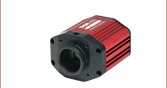
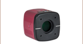
Mono., Passive Cooling: CS505MU Mono., Active Cooling: CC505MU Color: CS505CU Polarization: CS505MUP |
Mono.: CS895MU Color: CS895CU |
Mono.: CS126MU Color: CS126CU |
Monochrome, Passive Cooling: CS2100M-USB Active Cooling: CC215MU |
| Product Photos (Click to Enlarge) |
 |
 |
 |
||||
| Electronic Shutter | Global Shutter | Global Shutter | Rolling Shutterb | ||||
| Sensor Type | CMOS | CMOS | sCMOS | ||||
| Number of Pixels (H x V) |
1440 x 1080 | 1280 x 1024 | 1920 x 1200 | 2448 x 2048 | 4096 x 2160 | 4096 x 3000 | 1920 x 1080 |
| Pixel Size | 3.45 µm x 3.45 µm | 4.8 µm x 4.8 µm | 5.86 µm x 5.86 µm | 3.45 µm x 3.45 µm | 5.04 µm x 5.04 µm | ||
| Optical Format |
1/2.9" (6.2 mm Diag.) |
1/2" (7.76 mm Diag.) |
1/1.2" (13.4 mm Diag.) |
2/3" (11 mm Diag.) |
1" (16 mm Diag.) |
1.1" (17.5 mm Diag.) |
2/3" (11 mm Diag.) |
| Peak Quantum Efficiency (Click for Plot) |
Monochrome: 69% at 575 nm Color: Click for Plot |
Monochrome: 59% at 550 nm Color: Click for Plot NIR: 60% at 600 nm |
Monochrome: 78% at 500 nm Color: Click for Plot |
Monochrome & Polarization: 72% (525 to 580 nm) Color: Click for Plot |
Monochrome: 72% (525 to 580 nm) Color: Click for Plot |
Monochrome: 72% (525 to 580 nm) Color: Click for Plot |
Monochrome: 61% (at 600 nm) |
| Max Frame Rate (Full Sensor) |
34.8 fps | 92.3 fps | 39.7 fps | 35 fps | 20.8 fps | 14.6 fps | 50 fps |
| Read Noise | <4.0 e- RMS | <7.0 e- RMS | <7.0 e- RMS | <2.5 e- RMS | <1 e- Median RMS; <1.5 e- RMS | ||
| Digital Output |
10 Bit (Max) | 10 Bit (Max) | 12 Bit (Max) | 16 Bit (Max) | |||
| PC Interface | USB 3.0 | ||||||
| Available Fanless Cooling |
N/A | N/A | N/A | 0 °C at 20 °C Ambient (CC505MU Only) | N/A | 0 °C at 20 °C Ambient (CC215MU Only) |
|
| Housing Size (Click for Details) |
0.59" x 1.72" x 1.86" (15.0 x 43.7 x 47.2 mm3) |
Passively Cooled CMOS Camera TE-Cooled CMOS Camera |
Passively Cooled sCMOS Camera TE-Cooled sCMOS Camera |
||||
| Typical Applications |
General Purpose Imaging, Brightfield Microscopy, Machine Vision & Robotics, UAV, Drone, & Handheld Imaging, Inspection, Monitoring |
VIS/NIR Imaging, Electrophysiology/Brain Slice Imaging, Materials Inspection, Multispectral Imaging, Ophthalmology/Retinal Imaging, Vascular Imaging, Laser Speckle Imaging, Semiconductor Inspection, Fluorescence Microscopy, Brightfield Microscopy |
Fluorescence Microscopy, Immunohistochemistry, Machine Vision, Inspection, General Purpose Imaging |
Mono. & Color: Fluorescence Microscopy, Immunohistochemistry, Machine Vision & Inspection Polarization: Machine Vision & Inspection, Transparent Material Detection, Surface Reflection Reduction |
Fluorescence Microscopy, Immunohistochemistry, Large FOV Slide Imaging, Machine Vision, Inspection |
Fluorescence Microscopy, VIS/NIR Imaging, Quantum Dots, Autofluorescence, Materials Inspection, Multispectral Imaging |
|
| Scientific CCD Cameras | |||||||
|---|---|---|---|---|---|---|---|
| Camera Type | Fast Frame Rate VGA CCD |
1.4 MP CCD | 4 MP CCD | 8 MP CCD | |||
| Item # Prefix | Monochrome: 340M |
UV-Enhanced Monochrome: 340UV |
Monochrome: 1501M Color: 1501C |
Monochrome: 4070M Color: 4070C |
Monochrome: 8051M Color: 8051C |
Monochrome, No Sensor Face Plate: S805MU |
|
| Product Photo (Click to Enlarge) |
 |
 |
|
|
 |
||
| Electronic Shutter | Global Shutter | ||||||
| Sensor Type | CCD | ||||||
| Number of Pixels (H x V) |
640 x 480 | 1392 x 1040 | 2048 x 2048 | 3296 x 2472 | |||
| Pixel Size | 7.4 µm x 7.4 µm | 6.45 µm x 6.45 µm | 7.4 µm x 7.4 µm | 5.5 µm x 5.5 µm | |||
| Optical Format | 1/3" (5.92 mm Diagonal) | 2/3" (11 mm Diagonal) | 4/3" (21.4 mm Diagonal) | 4/3" (22 mm Diagonal) | |||
| Peak QE (Click for Plot) |
55% at 500 nm |
10% at 485 nm |
Monochrome: 60% at 500 nm Color: Click for Plot |
Monochrome: 52% at 500 nm Color: Click for Plot |
Monochrome: 51% at 460 nm Color: Click for Plot |
51% at 460 nm | |
| Max Frame Rate (Full Sensor) |
200.7 fps (at 40 MHz Dual-Tap Readout) |
23 fps (at 40 MHz Single-Tap Readout) |
25.8 fps (at 40 MHz Quad-Tap Readout)a |
17.1 fps (at 40 MHz Quad-Tap Readout)b |
17.1 fps (at 40 MHz Quad-Tap Readout) |
||
| Read Noise | <15 e- at 20 MHz | <7 e- at 20 MHz (Standard Models) <6 e- at 20 MHz (-TE Models) |
<12 e- at 20 MHz | <10 e- at 20 MHz | |||
| Digital Output (Max) | 14 Bitc | 14 Bit | 14 Bitc | 14 Bit | |||
| Available Fanless Cooling |
Passive Thermal Management | -20 °C at 20 °C Ambient Temperature | -10 °C at 20 °C Ambient | Passive Thermal Management | |||
| Available PC Interfaces |
USB 3.0 or Gigabit Ethernet | USB 3.0 | |||||
| Housing Dimensions (Click for Details) |
Non-Cooled Scientific CCD Camera |
Cooled Scientific CCD Camera Non-Cooled Scientific CCD Camera |
No Face Plate Scientific CCD Camera |
||||
| Typical Applications | Ca++ Ion Imaging, Particle Tracking, Flow Cytometry, SEM/EBSD, UV Inspection |
Fluorescence Microscopy, VIS/NIR Imaging, Quantum Dots, Multispectral Imaging, Immunohistochemistry (IHC), Retinal Imaging |
Fluorescence Microscopy, Transmitted Light Microscopy, Whole-Slide Microscopy, Electron Microscopy (TEM/SEM), Inspection, Material Sciences |
Fluorescence Microscopy, Whole-Slide Microscopy, Large FOV Slide Imaging, Histopathology, Inspection, Multispectral Imaging, Immunohistochemistry (IHC) |
Beam Profiling & Characterization, Interferometry, VCSEL Inspection, Quantitative Phase-Contrast Microscopy, Ptychography, Digital Holographic Microscopy |
||

 Zoom
Zoom
Click for Details
A schematic showing a TSI-IOBOB2 connected to an Arduino to trigger a compact scientific camera.


These optional accessories allow for easy use of the auxiliary port of our compact scientific (sCMOS & CMOS) or scientific CCD cameras. These items should be considered when it is necessary to externally trigger the camera, to monitor camera performance with an oscilloscope, or for simultaneous control of the camera with other instruments.
For our USB 3.0 cameras, we also offer a PCIe USB 3.0 card and extra cables for facilitating the connection to the computer.
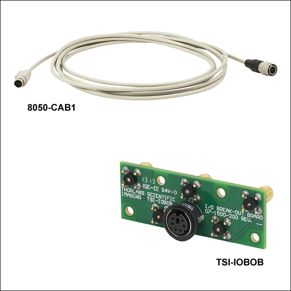
Auxiliary I/O Cable (8050-CAB1)
The 8050-CAB1 is a 10' (3 m) long cable that mates with the auxiliary connector on our scientific cameras* and provides the ability to externally trigger the camera as well as monitor status output signals. One end of the cable features a male 12-pin connector for connecting to the camera, while the other end has a male 6-pin Mini Din connector for connecting to external devices. This cable is ideal for use with our interconnect break-out boards described below. For information on the pin layout, please see the Pin Diagrams tab above.
*The 8050-CAB1 cable is not compatible with our former-generation 1500M series cameras.
Interconnect Break-Out Board (TSI-IOBOB)
The TSI-IOBOB is designed to "break out" the 6-pin Mini Din connector found on our scientific camera auxiliary cables into five SMA connectors. The SMA connectors can then be connected using SMA cables to other devices to provide a trigger input to the camera or to monitor camera performance. The pin configurations are listed on the Pin Diagrams tab above.
Interconnect Break-Out Board / Shield for Arduino (TSI-IOBOB2)
The TSI-IOBOB2 offers the same breakout functionality of the camera signals as the TSI-IOBOB. Additionally, it functions as a shield for Arduino, by placing the TSI-IOBOB2 shield on a Arduino board supporting the Arduino Uno Rev. 3 form factor. While the camera inputs and outputs are 5 V TTL, the TSI-IOBOB2 features bi-directional logic level converters to enable compatibility with Arduino boards operating on either 5 V or 3.3 V logic. Sample programs for controlling the scientific camera are available for download from our software page, and are also described in the manual (found by clicking on the red Docs icon below). For more information on Arduino, or for information on purchasing an Arduino board, please see www.arduino.cc.
The image to the right shows a schematic of a configuration with the TSI-IOBOB2 with an Arduino board integrated into a camera imaging system. The camera is connected to the break-out board using a 8050-CAB1 cable that must be purchased separately. The pins on the shield can be used to deliver signals to simultaneously control other peripheral devices, such as light sources, shutters, or motion control devices. Once the control program is written to the Arduino board, the USB connection to the host PC can be removed, allowing for a stand-alone system control platform; alternately, the USB connection can be left in place to allow for two-way communication between the Arduino and the PC. The compact size of 2.70" x 2.10" (68.6 mm x 53.3 mm) also aids in keeping systems based on the TSI-IOBOB2 compact.
USB 3.0 Camera Accessories (USB3-MBA-118 and USB3-PCIE)
We also offer a USB 3.0 A to Micro B cable for connecting our cameras to a PC. Please note that one USB3-MBA-118 cable is included with each USB 3.0 camera except the CC215MU cooled Quantalux camera. The CC215MU camera ships with an appropriate USB 3.0 cable and should not be used with the USB3-MBA-118. The USB3-MBA-118 cable measures 118" long and features screws on either side of the Micro B connector that mate with tapped holes on the camera for securing the USB cable to the camera housing. When operating USB 3.0 cameras it is strongly recommended that the Thorlabs-supplied USB 3.0 cable be used, with the retention screws securely fastened. Due to the high data rates involved, users may experience problems when using generic USB 3.0 cables.
Cameras with USB 3.0 connectivity may be connected directly to the USB 3.0 port on a laptop or desktop computer. USB 3.0 cameras are not compatible with USB 2.0 ports. Host-side USB 3.0 ports are often blue in color, although they may also be black in color, and typically marked "SS" for SuperSpeed. A USB 3.0 PCIe card is sold separately for computers without an integrated Intel USB 3.0 controller. Note that the use of a USB hub may impact performance. A dedicated connection to the PC is preferred.

 Zoom
Zoom
The SM1A10A is a replacement SM1 to C-Mount adapter for the non-cooled Kiralux® and Quantalux® cameras. This adapter has external SM1 (1.035"-40) threads and internal C-Mount (1.00"-32) threads for compatibility with many microscopes, machine vision camera lenses, and C-Mount extension tubes. The adapter also comes with a SM1NT locking ring.