 Products Home / Polarization Optics / Liquid Crystal Devices / Liquid Crystal Optical Beam Shutter / Variable Attenuator
Liquid Crystal Optical Beam Shutter / Variable Attenuator

- Vibration Free with Fast Shutter Switching Speeds: ≤5 ms
- High Transmission and High Contrast Ratio
of Visible Wavelengths (420 - 700 nm) - Optical Shutter and Variable Attenuator Modes
LCC1620
Liquid Crystal Optical Shutter
Application Idea
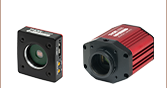
LCC1620 Optical Shutter Mounted to a
1500M-GE-TE 1.4 Megapixel Scientific
CCD Camera with an SM1A39 Adapter


Please Wait

Click to Enlarge
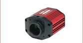
The front face of the LCC1620 shutter head. Both the back and front of the shutter are engraved with the transmission axis and both feature internal SM1 threads.

Click to Enlarge
The graph above shows the measured transmission through the shutter and contrast ratio as a function of wavelength. The shaded regions denote the wavelength range over which we guarantee the shutter will meet the specifications listed in the Specs tab. Performance outside the shaded regions will vary from lot to lot and is not guaranteed. For a raw data file and additional plots, please see the Graphs tab.

Click to Enlarge
The side view of the LCC1620 Liquid Crystal Shutter, showing the STATUS LED light and power connector.
Features
- Liquid Crystal Optical Shutter and Variable Attenuator for 420 - 700 nm Light
- Vibration-Free Device with No Moving Parts
- High Average Transmittance (>60%) and Contrast Ratio (8000:1) Over Operating Wavelength Range
- Shutter and Attenuator Modes
- Fast Shutter Switching Speeds (Shutter Mode):
- Opening: 5 ms
- Closing: 1 ms
- Post Mountable and 30 mm Cage System Compatible
- SM1 (1.035"-40) Threaded for Compatibility with Lens Tubes
Thorlabs’ Liquid Crystal (LC) Optical Shutter / Variable Attenuator incorporates a liquid crystal cell sandwiched between polarizing elements that is used to quickly change the transmission to either block or attenuate light propagating through the device. The shutter operates over the 420 to 700 nm wavelength range. The LCC1620(/M) optical shutter provides rapid and vibrationless (due to no moving parts) control over the intensity of light through the device. Due to its rapid switching capabilities, this LC optical shutter is ideal for imaging and precision illumination applications. It can be used either as an optical shutter to block/transmit a beam or as a variable attenuator. In shutter mode, it can open in 5 ms and close in 1 ms (see the Specs tab for more information). When in attenuator mode, the potentiometer on top of the shutter is used to set the attenuation level.
A switch on the top of the shutter allows the user to select the shutter or attenuator mode. In the shutter mode, the LCC1620 will act similarly to a mechanical shutter, either allowing the light through or blocking it completely. In the attenuator mode it will act as a variable attenuator with the attenuation level controlled by the knob on the top of the shutter. The shutter can be controlled, in both modes, manually by adjusting the knob on the top of the shutter or through an external signal via the SMC connector. In Shutter mode this external signal is a 0 - 5 V TTL signal, in Attenuator mode this external signal is a 0 - 5 V DC signal. An LED on the side of the shutter (labeled "STATUS") will indicate green when the shutter is transmitting light and red when it is completely blocking light.
This LC Shutter is capable of achieving switching speeds that are significantly faster than either our single-blade or diaphragm optical beam shutters. Additionally, it can be modulated to higher frequencies than either of the mechanical shutters. However, due to the wavelength limitations of the liquid crystal cells, for applications above 700 nm or below 420 nm, the mechanical shutters should be used instead. The mechanical shutters should also be considered for applications that require unpolarized light since the LC shutter utilizes polarizers as part of the liquid crystal cell design.
Transmission & Polarization
Because the LC shutter is made from liquid crystal cells and polarizers, it is not sensitive to the direction of propagation and may be used in either direction. However, each face is engraved with a white line (see image above) that indicates the polarization axis for the device. For maximum transmission, the input beam should be linearly polarized and aligned with the polarization axis of the shutter. It should be noted, however, that the shutter will rotate the polarization axis by 90° at the output. The shutter is compatible with unpolarized light, however, due to the polarizers inside the device, the total transmission will be greatly reduced (since half the light will be blocked by the first polarizer).
Mounting Options
The front and back faces of the housing are SM1 (1.035"-40) threaded, which is ideal for mounting filters or Ø1" lens tubes to the housing. Additionally, four 4-40 tapped holes on the front and back faces ensure compatibility with Thorlabs' 30 mm cage system. These shutters are post mountable via one of two 8-32 (M4) taps on the sides of the housing.
| Item # | LCC1620(/M) | |
|---|---|---|
| Operating Wavelength Range | 420 - 700 nm | |
| Transmissiona (Shutter Mode, Avg.) | >60% | |
| Contrast Ratiob (Avg.) | >8000:1 | |
| Laser Damage Threshold | CWc | 1 W/cm2 (532 nm, Ø0.471 mm) |
| Pulsed (ns) | 0.4 J/cm2 (532 nm, 10 ns, 10 Hz, Ø0.750 mm) | |
| Clear Aperture | Ø20 mm | |
| Surface Quality | 40-20 Scratch-Dig | |
| Max Incidence Angle | ±5° | |
| Switching Speed (in Shutter Mode)d | Opening: 5 ms (Typ.) Closing: 1 ms (Typ.) |
|
| Operating Frequency Rangee | 0 - 50 Hz | |
| Wavefront Distortion | ≤λ/4 @ 633 nm | |
| External Input | SMC Connector, 0 - 5 V, 25 kΩ Input Impedance | |
| Power Adapter | 12 VDC / 1.25 A with Power Cord | |
| AC Power Requirements | 110 - 240 VAC, 47 - 63 Hz, 0.4 A | |
| Mounting | Two #8-32 (M4) Threaded Holes for Post Mounting 30 mm Cage System Compatible Ø1" Lens Tube Compatible |
|
| Operating Temperature | 15 to 60 °C | |
| Dimension (L × W × H) | 60 × 27 × 60 mm (2.36" × 1.06" × 2.36") |
|

Click to Enlarge
The above is a diagram showing the timing of a TTL pulse (top) and the shutter response (bottom).
| Shutter Timing Specifications | ||
|---|---|---|
| Diagram Keya | Description | Time (Typ.) |
| A-B | Delay between the input pulse's rising edge at 90% and the initialization of shutter down to 90% | 0.065 ms |
| B-C | Falling edge from 90% to 10% | 0.346 ms |
| A-C | Delay between the input pulse's rising edge at 90% and shutter down to 10% | 0.416 ms |
| D-E | Delay between the input pulse's falling edge at 10% and initialization of the shutter rise to 10% | 2.23 ms |
| E-F | Rising Edge from 10% to 90% | 3.24 ms |
| D-F | Delay between the input pulse's falling edge at 10% and shutter rise to 90% | 5.47 ms |
The graphs below represent the measured data sets for the LCC1620(/M) LC Optical Shutter. All data was obtained with linearly polarized light with the axis of polarization aligned to the transmission axis (marked by a white line on the face) of the shutter. The contrast ratio is defined as the ratio of the transmitted light when the shutter is open to the transmitted light when the shutter is closed.

Click to Enlarge
Click for Raw Data
The graph above shows the measured transmission through the shutter as a function of attenuation voltage, taken in Attenuator Mode. The attenuation voltage was set by an external voltage. Data for multiple wavelengths are shown.

Click to Enlarge
Click for Raw Data
The graph above shows the measured transmission through the shutter as a function of wavelength, taken in Attenuator Mode with the voltage set by an external source. Data for multiple attenuation voltages are shown.

Click to Enlarge
Click for Raw Data
The graph above shows the measured transmission through the shutter as a function of wavelength. Data for multiple temperatures are shown.

Click to Enlarge
Click for Raw Data
The graph above shows the measured transmission through the shutter as a function of wavelength. Data for multiple Angles of Incidence (AOI) are shown.

Click to Enlarge
Click for Raw Data
The graph above shows the measured contrast ratio of the shutter as a function of wavelength. The contrast ratio is defined as the ratio of the transmitted light when the shutter is open to the transmitted light when the shutter is closed. Data for multiple temperatures are shown.

Click to Enlarge
Click for Raw Data
The graph above shows the measured contrast ratio of the shutter as a function of wavelength. The contrast ratio is defined as the ratio of the transmitted light when the shutter is open to the transmitted light when the shutter is closed. Data for multiple Angles of Incidence (AOI) are shown.

Click to Enlarge
Click for Raw Data
The graph above shows the measured transmission through the shutter and contrast ratio as a function of wavelength taken at 25 °C. The contrast ratio is defined as the ratio of the transmitted light when the shutter is open to the transmitted light when the shutter is closed.

Click to Enlarge
Click for Raw Data
The graph above shows the measured normalized transmission through the shutter over a 20 hour period.

Click to Enlarge
The graph above shows the measured contrast ratio of the shutter as a function of frequency. The contrast ratio is defined as the ratio of the transmitted light when the shutter is open to the transmitted light when the shutter is closed.

Click to Enlarge
The graph above shows the stability of the shutter switching time over a 6 week period.
| Damage Threshold Specifications | |
|---|---|
| Laser Type | Damage Threshold |
| Pulsed (ns) | 0.4 J/cm2 (532 nm, 10 ns, 10 Hz, Ø0.750 mm) |
| CWa | 1 W/cm2 (532 nm, Ø0.471 mm) |
Damage Threshold Data for Thorlabs' LC Shutters
The specifications to the right are measured data for Thorlabs' Liquid Crystal Shutter.
Laser Induced Damage Threshold Tutorial
The following is a general overview of how laser induced damage thresholds are measured and how the values may be utilized in determining the appropriateness of an optic for a given application. When choosing optics, it is important to understand the Laser Induced Damage Threshold (LIDT) of the optics being used. The LIDT for an optic greatly depends on the type of laser you are using. Continuous wave (CW) lasers typically cause damage from thermal effects (absorption either in the coating or in the substrate). Pulsed lasers, on the other hand, often strip electrons from the lattice structure of an optic before causing thermal damage. Note that the guideline presented here assumes room temperature operation and optics in new condition (i.e., within scratch-dig spec, surface free of contamination, etc.). Because dust or other particles on the surface of an optic can cause damage at lower thresholds, we recommend keeping surfaces clean and free of debris. For more information on cleaning optics, please see our Optics Cleaning tutorial.
Testing Method
Thorlabs' LIDT testing is done in compliance with ISO/DIS 11254 and ISO 21254 specifications.
First, a low-power/energy beam is directed to the optic under test. The optic is exposed in 10 locations to this laser beam for 30 seconds (CW) or for a number of pulses (pulse repetition frequency specified). After exposure, the optic is examined by a microscope (~100X magnification) for any visible damage. The number of locations that are damaged at a particular power/energy level is recorded. Next, the power/energy is either increased or decreased and the optic is exposed at 10 new locations. This process is repeated until damage is observed. The damage threshold is then assigned to be the highest power/energy that the optic can withstand without causing damage. A histogram such as that below represents the testing of one BB1-E02 mirror.

The photograph above is a protected aluminum-coated mirror after LIDT testing. In this particular test, it handled 0.43 J/cm2 (1064 nm, 10 ns pulse, 10 Hz, Ø1.000 mm) before damage.

| Example Test Data | |||
|---|---|---|---|
| Fluence | # of Tested Locations | Locations with Damage | Locations Without Damage |
| 1.50 J/cm2 | 10 | 0 | 10 |
| 1.75 J/cm2 | 10 | 0 | 10 |
| 2.00 J/cm2 | 10 | 0 | 10 |
| 2.25 J/cm2 | 10 | 1 | 9 |
| 3.00 J/cm2 | 10 | 1 | 9 |
| 5.00 J/cm2 | 10 | 9 | 1 |
According to the test, the damage threshold of the mirror was 2.00 J/cm2 (532 nm, 10 ns pulse, 10 Hz, Ø0.803 mm). Please keep in mind that these tests are performed on clean optics, as dirt and contamination can significantly lower the damage threshold of a component. While the test results are only representative of one coating run, Thorlabs specifies damage threshold values that account for coating variances.
Continuous Wave and Long-Pulse Lasers
When an optic is damaged by a continuous wave (CW) laser, it is usually due to the melting of the surface as a result of absorbing the laser's energy or damage to the optical coating (antireflection) [1]. Pulsed lasers with pulse lengths longer than 1 µs can be treated as CW lasers for LIDT discussions.
When pulse lengths are between 1 ns and 1 µs, laser-induced damage can occur either because of absorption or a dielectric breakdown (therefore, a user must check both CW and pulsed LIDT). Absorption is either due to an intrinsic property of the optic or due to surface irregularities; thus LIDT values are only valid for optics meeting or exceeding the surface quality specifications given by a manufacturer. While many optics can handle high power CW lasers, cemented (e.g., achromatic doublets) or highly absorptive (e.g., ND filters) optics tend to have lower CW damage thresholds. These lower thresholds are due to absorption or scattering in the cement or metal coating.

LIDT in linear power density vs. pulse length and spot size. For long pulses to CW, linear power density becomes a constant with spot size. This graph was obtained from [1].

Pulsed lasers with high pulse repetition frequencies (PRF) may behave similarly to CW beams. Unfortunately, this is highly dependent on factors such as absorption and thermal diffusivity, so there is no reliable method for determining when a high PRF laser will damage an optic due to thermal effects. For beams with a high PRF both the average and peak powers must be compared to the equivalent CW power. Additionally, for highly transparent materials, there is little to no drop in the LIDT with increasing PRF.
In order to use the specified CW damage threshold of an optic, it is necessary to know the following:
- Wavelength of your laser
- Beam diameter of your beam (1/e2)
- Approximate intensity profile of your beam (e.g., Gaussian)
- Linear power density of your beam (total power divided by 1/e2 beam diameter)
Thorlabs expresses LIDT for CW lasers as a linear power density measured in W/cm. In this regime, the LIDT given as a linear power density can be applied to any beam diameter; one does not need to compute an adjusted LIDT to adjust for changes in spot size, as demonstrated by the graph to the right. Average linear power density can be calculated using the equation below.

The calculation above assumes a uniform beam intensity profile. You must now consider hotspots in the beam or other non-uniform intensity profiles and roughly calculate a maximum power density. For reference, a Gaussian beam typically has a maximum power density that is twice that of the uniform beam (see lower right).
Now compare the maximum power density to that which is specified as the LIDT for the optic. If the optic was tested at a wavelength other than your operating wavelength, the damage threshold must be scaled appropriately. A good rule of thumb is that the damage threshold has a linear relationship with wavelength such that as you move to shorter wavelengths, the damage threshold decreases (i.e., a LIDT of 10 W/cm at 1310 nm scales to 5 W/cm at 655 nm):

While this rule of thumb provides a general trend, it is not a quantitative analysis of LIDT vs wavelength. In CW applications, for instance, damage scales more strongly with absorption in the coating and substrate, which does not necessarily scale well with wavelength. While the above procedure provides a good rule of thumb for LIDT values, please contact Tech Support if your wavelength is different from the specified LIDT wavelength. If your power density is less than the adjusted LIDT of the optic, then the optic should work for your application.
Please note that we have a buffer built in between the specified damage thresholds online and the tests which we have done, which accommodates variation between batches. Upon request, we can provide individual test information and a testing certificate. The damage analysis will be carried out on a similar optic (customer's optic will not be damaged). Testing may result in additional costs or lead times. Contact Tech Support for more information.
Pulsed Lasers
As previously stated, pulsed lasers typically induce a different type of damage to the optic than CW lasers. Pulsed lasers often do not heat the optic enough to damage it; instead, pulsed lasers produce strong electric fields capable of inducing dielectric breakdown in the material. Unfortunately, it can be very difficult to compare the LIDT specification of an optic to your laser. There are multiple regimes in which a pulsed laser can damage an optic and this is based on the laser's pulse length. The highlighted columns in the table below outline the relevant pulse lengths for our specified LIDT values.
Pulses shorter than 10-9 s cannot be compared to our specified LIDT values with much reliability. In this ultra-short-pulse regime various mechanics, such as multiphoton-avalanche ionization, take over as the predominate damage mechanism [2]. In contrast, pulses between 10-7 s and 10-4 s may cause damage to an optic either because of dielectric breakdown or thermal effects. This means that both CW and pulsed damage thresholds must be compared to the laser beam to determine whether the optic is suitable for your application.
| Pulse Duration | t < 10-9 s | 10-9 < t < 10-7 s | 10-7 < t < 10-4 s | t > 10-4 s |
|---|---|---|---|---|
| Damage Mechanism | Avalanche Ionization | Dielectric Breakdown | Dielectric Breakdown or Thermal | Thermal |
| Relevant Damage Specification | No Comparison (See Above) | Pulsed | Pulsed and CW | CW |
When comparing an LIDT specified for a pulsed laser to your laser, it is essential to know the following:

LIDT in energy density vs. pulse length and spot size. For short pulses, energy density becomes a constant with spot size. This graph was obtained from [1].
- Wavelength of your laser
- Energy density of your beam (total energy divided by 1/e2 area)
- Pulse length of your laser
- Pulse repetition frequency (prf) of your laser
- Beam diameter of your laser (1/e2 )
- Approximate intensity profile of your beam (e.g., Gaussian)
The energy density of your beam should be calculated in terms of J/cm2. The graph to the right shows why expressing the LIDT as an energy density provides the best metric for short pulse sources. In this regime, the LIDT given as an energy density can be applied to any beam diameter; one does not need to compute an adjusted LIDT to adjust for changes in spot size. This calculation assumes a uniform beam intensity profile. You must now adjust this energy density to account for hotspots or other nonuniform intensity profiles and roughly calculate a maximum energy density. For reference a Gaussian beam typically has a maximum energy density that is twice that of the 1/e2 beam.
Now compare the maximum energy density to that which is specified as the LIDT for the optic. If the optic was tested at a wavelength other than your operating wavelength, the damage threshold must be scaled appropriately [3]. A good rule of thumb is that the damage threshold has an inverse square root relationship with wavelength such that as you move to shorter wavelengths, the damage threshold decreases (i.e., a LIDT of 1 J/cm2 at 1064 nm scales to 0.7 J/cm2 at 532 nm):

You now have a wavelength-adjusted energy density, which you will use in the following step.
Beam diameter is also important to know when comparing damage thresholds. While the LIDT, when expressed in units of J/cm², scales independently of spot size; large beam sizes are more likely to illuminate a larger number of defects which can lead to greater variances in the LIDT [4]. For data presented here, a <1 mm beam size was used to measure the LIDT. For beams sizes greater than 5 mm, the LIDT (J/cm2) will not scale independently of beam diameter due to the larger size beam exposing more defects.
The pulse length must now be compensated for. The longer the pulse duration, the more energy the optic can handle. For pulse widths between 1 - 100 ns, an approximation is as follows:

Use this formula to calculate the Adjusted LIDT for an optic based on your pulse length. If your maximum energy density is less than this adjusted LIDT maximum energy density, then the optic should be suitable for your application. Keep in mind that this calculation is only used for pulses between 10-9 s and 10-7 s. For pulses between 10-7 s and 10-4 s, the CW LIDT must also be checked before deeming the optic appropriate for your application.
Please note that we have a buffer built in between the specified damage thresholds online and the tests which we have done, which accommodates variation between batches. Upon request, we can provide individual test information and a testing certificate. Contact Tech Support for more information.
[1] R. M. Wood, Optics and Laser Tech. 29, 517 (1998).
[2] Roger M. Wood, Laser-Induced Damage of Optical Materials (Institute of Physics Publishing, Philadelphia, PA, 2003).
[3] C. W. Carr et al., Phys. Rev. Lett. 91, 127402 (2003).
[4] N. Bloembergen, Appl. Opt. 12, 661 (1973).
| Posted Comments: | |
Xiaoya Su
(posted 2020-03-23 05:32:07.623) Dear Sir/Madam,
I have seen in your specs that the damage threshold is scaled in W/cm2, but in the introduction of calculation method of damage threshold, it says 'Thorlabs expresses LIDT for CW lasers as a linear power density measured in W/cm'. So which one eventually should I refer to?
Thanks and looking forward to your reply.
Yours sincerely,
Xiaoya Su YLohia
(posted 2020-03-24 09:25:40.0) Hello Xiaoya, thank you for contacting Thorlabs. The damage threshold for this item was characterized in the past when we still measured this parameter in W/cm^2. The footnote you saw is intended to be paired with our specs that are given in W/cm across our various product pages on the website. Thank you for bringing this to our attention. We will work on correcting this. For your application, please refer to the W/cm^2 measurement as this is the data we currently have. mawenjin Ma
(posted 2019-06-03 09:51:02.15) Dear tholarbs:
Whether there is threshold voltage in shutter mode?Can we apply the voltage exceed 5 V in shutter mode? YLohia
(posted 2019-06-03 03:02:08.0) Hello, thank you for contacting Thorlabs. When operating in "Shutter Mode" we recommend the Voltage IN to be between 4.8V-5V (closed) and 0V-1V (open). We do not recommend going over the 5V max. emilio
(posted 2017-10-28 00:15:07.55) Wish it was available in NIR. nbayconich
(posted 2017-11-20 08:25:24.0) Thank you for contacting Thorlabs. We can provide customized versions of these liquid crystal shutters in NIR. I will contact you directly with more information about our custom capabilities. |
| Shutter Selection Guide | ||||
|---|---|---|---|---|
| Shutter Type | Liquid Crystal | Mechanical | ||
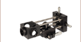
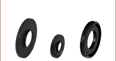
| Single Blade | Diaphragm | Mechanical Chopper | ||
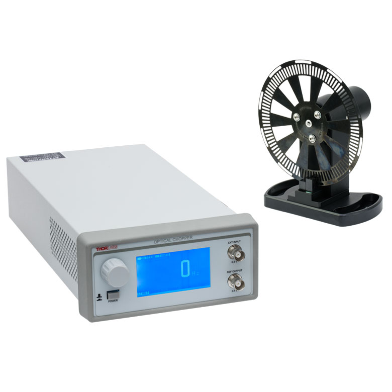
| Sample Product Photo (Click to Enlarge) |
 |
 |
 |
 |
| Modulation Frequency | Up to 50 Hz | Continuous: Up to 10 Hz Burst: Up to 25 Hz |
Continuous: Up to 15 Hz Burst: Up to 50 Hz |
Up to 10 kHz (Depending on Blade) |
| Variable Attenuation | Yes | No | No | No |
| Custom Modulation | Triggered and Analog | Triggered | Triggered | Controlled by Chopper Speed, Always Periodic |
| 100% Transmission | No | Yes | Yes | Yes |
| 100% Attenuation | No | Yes | Yes | Yes |
| Clear Aperture | Ø20 mm | Ø1/2" or Ø1" | Ø1/4", Ø1/2", or Ø1" | Dependent on Chopper Blade |
| Vibration/Noise Free | Yes | No | No | No |
| Integration Features | SM1-Threaded Aperture, 30 mm Cage Compatible, and Tap for Post Mounting |
SM05- or SM1-Threaded Aperture, 30 mm Cage Compatible, and Tap for Post Mounting |
SM05- or SM1-Threaded Aperture; Adapters for 30 mm Cage System or Post Mounting |
Stand for Chopper Wheel (Included) |